Author: Denis Avetisyan
New research reveals that apparent price jumps at the highest data frequencies are largely explained by intense bursts of volatility, challenging conventional understandings of market behavior.
Analysis of ultra-high-frequency tick data demonstrates that the true jump component in asset prices is significantly smaller than previously estimated using lower-frequency measurements.
Conventional analyses of financial time series often overestimate the prevalence of discrete price jumps, leading to mischaracterizations of market behavior. This paper, ‘Fact or friction: Jumps at ultra high frequency’, leverages millisecond-precision tick data and novel econometric techniques to reassess the contribution of jumps to overall price variation. Our findings demonstrate that the true magnitude of jump variation is likely an order of magnitude smaller than previously reported, with many apparent jumps attributable to bursts of high-frequency volatility. Ultimately, this raises the question of whether existing models adequately capture the nuanced dynamics of price discovery at the most granular levels.
Unveiling Hidden Patterns: The Limits of Continuous Models
For decades, the prevailing framework in financial modeling has centered on continuous-time diffusion processes, most notably the Random Walk, to depict asset price evolution. This approach inherently assumes that price changes occur gradually and smoothly, mirroring the physics of Brownian motion. The Random Walk, and its more complex derivatives, posit that price fluctuations are the result of an infinite series of infinitely small, random increments. While mathematically tractable and computationally convenient, this reliance on continuous processes represents a simplification of real-world market dynamics. It allows for elegant theoretical results and provides a foundation for many derivative pricing formulas, but it struggles to fully capture the often-observed reality of sudden, discontinuous price shifts that characterize financial markets. This foundational assumption, though useful, necessitates careful consideration when applied to empirical data, as it may overlook important features of price formation.
Traditional financial modeling often assumes asset prices evolve through continuous processes, akin to a smooth, uninterrupted random walk. However, empirical observation of financial markets reveals a different reality – prices don’t merely drift, they frequently jump. These abrupt shifts, driven by unexpected news, macroeconomic shocks, or even investor sentiment, represent discrete changes that deviate significantly from the predictions of continuous models. The prevalence of these jumps poses a challenge for accurately capturing price dynamics, as standard asset pricing techniques can underestimate the true volatility and risk inherent in financial instruments. Consequently, failing to account for these discontinuities can lead to miscalculations in derivative pricing and flawed assessments of potential losses, highlighting the need for methodologies that explicitly incorporate the impact of these sudden price movements.
The reliance on continuous diffusion models in finance carries significant implications for derivative pricing and risk assessment. When abrupt price changes – discontinuities, or ‘jumps’ – are disregarded, option valuations can deviate substantially from their true values, leading to potential losses for investors and institutions. Similarly, risk management strategies predicated on the assumption of smooth price movements may underestimate the likelihood of extreme events and fail to adequately protect against substantial declines. This underestimation can result in insufficient capital reserves and an inaccurate assessment of portfolio vulnerability. Consequently, a precise understanding and incorporation of these price discontinuities are not merely academic refinements, but essential components of sound financial modeling and effective risk mitigation.
Accurate financial modeling increasingly relies on the precise measurement of price discontinuities, often termed ‘jumps’, within asset time series. While traditional approaches often assume continuous price movements, modern analysis reveals that these abrupt shifts, though frequent, contribute surprisingly little to overall price variation. Recent investigations into high-frequency equity and foreign exchange data demonstrate that the jump component typically accounts for only around 1% of total price variability – a significantly lower figure than previously estimated. This finding has important implications for derivative pricing, where jump diffusion models are employed, and for risk management strategies that depend on accurately quantifying potential price shocks. Consequently, developing robust methodologies for identifying and quantifying this jump variation remains crucial for modern financial analysis and building more reliable predictive models.
Refining the Signal: Data Preparation for Accuracy
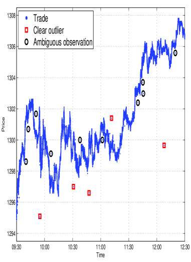
High-frequency financial data, commonly referred to as Tick Data, is characterized by a large volume of transactions recorded at very short intervals. This granularity, while providing detailed insights, also introduces inherent noise due to factors like order book dynamics, latency in data capture, and data transmission errors. Specifically, the data frequently contains outliers – values significantly deviating from the expected range – and erratic fluctuations that do not reflect genuine price movements. These anomalies arise from various sources including erroneous trades, stale quotes, and split-second discrepancies in timestamping. Consequently, without appropriate pre-processing, analyses based directly on raw Tick Data can yield inaccurate results and misleading interpretations of market behavior, necessitating robust filtering and cleaning techniques.
The initial data preparation stage necessitates the application of a Bid-Ask Mid-Price (BMF) Filter to synchronize trade and quote data, addressing discrepancies arising from asynchronous recording. This filter calculates the mid-price as (Bid + Ask) / 2 and uses it as a reference point to align trades that fall between bid and ask prices. Following BMF filtering, Outlier Filtering is implemented to identify and remove erroneous data points, typically based on statistical measures such as standard deviation or interquartile range. Values exceeding predefined thresholds – indicating likely errors or data transmission issues – are either removed or flagged for further investigation, ensuring the integrity of the dataset prior to subsequent analysis.
Pre-averaging techniques in financial data preparation involve calculating the mean of data points within defined time intervals, typically ranging from several seconds to minutes, to create a smoothed time series. This process reduces the impact of individual noisy data points – such as errant ticks or temporary imbalances – by replacing them with the average value over the specified window. Common methods include Simple Moving Averages (SMA) and Exponential Moving Averages (EMA), each differing in how they weight older data points. The selection of the averaging window length is crucial; shorter windows preserve more high-frequency information but offer less noise reduction, while longer windows provide greater smoothing but can obscure important price movements. The resulting pre-averaged data then serves as a more stable foundation for subsequent analysis, including volatility calculations, trend identification, and algorithmic trading strategies.
The application of data cleaning techniques – including Bid-Ask Midpoint Filtering and Outlier Removal – is fundamental to accurate price variation analysis. Raw financial data frequently contains errors and inconsistencies that, if left unaddressed, will disproportionately influence statistical calculations. By systematically identifying and mitigating these spurious fluctuations, the process establishes a dataset where observed price movements reflect genuine market signals rather than data anomalies. This is critical for reliable backtesting, algorithmic trading strategy development, and the calculation of volatility metrics, as the integrity of these analyses is directly dependent on the quality of the underlying data.
Dissecting Variation: Methods for Quantifying Jumps
Estimating jump variation requires consideration of multiple methodologies, each exhibiting trade-offs between computational complexity, sensitivity to noise, and accuracy. Early approaches, such as the Press model, relied on simplified assumptions about the distribution of price changes and are susceptible to bias in the presence of frequent, small jumps. More sophisticated estimators, including the Barndorff-Nielsen & Shephard bi-power variation, incorporate techniques to mitigate the impact of microstructure noise and provide more robust estimates, but at the cost of increased computational demands. Realized Variation, while a fundamental measure of total variation, does not inherently distinguish between continuous and jump components and is therefore often paired with jump-robust estimators. The selection of an appropriate method depends on the specific characteristics of the data, the desired level of accuracy, and the available computational resources.
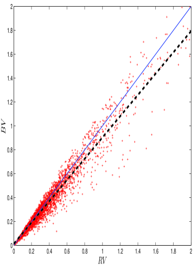
The Press Model, an early estimator of quadratic variation, operates by summing squared price changes over a specified time interval, effectively approximating the total variation in price. However, this approach is sensitive to market microstructure noise and can misidentify noise as genuine price jumps. Subsequent advancements, notably the Barndorff-Nielsen & Shephard (BNS) Bi-Power Variation estimator, address these limitations through the incorporation of a weighting scheme designed to reduce the impact of noisy high-frequency data. The BNS estimator utilizes the concept of realized bi-power variation, calculated as \sum_{i=1}^{n-1} (R_{i+1} - R_i)^2, where R_i represents the logarithmic price at time i, and applies a correction factor to improve its consistency and reduce bias in the presence of jumps. This results in a more robust estimation of the true underlying variation, particularly in volatile market conditions.
Realized Variation (RV) is a widely used estimator of the quadratic variation of a continuous semimartingale, calculated as the sum of squared returns over a specified time interval. Specifically, RV is computed as \sum_{i=1}^{n} r_{i}^2, where r_{i} represents the return between time points t_{i-1} and t_{i}. While RV effectively captures total price variation under the assumption of continuous paths, its accuracy diminishes in the presence of jumps. Consequently, RV is frequently employed in conjunction with jump-robust estimators – methods designed to specifically isolate and account for discontinuous price movements – to provide a more comprehensive and accurate assessment of total variation by separating continuous and jump components. This combined approach enhances the reliability of volatility estimates and facilitates more precise financial modeling.
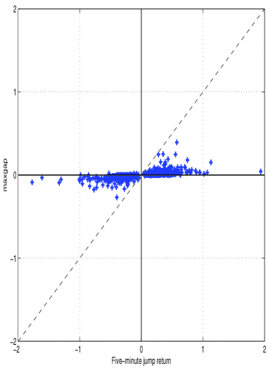
The Maxgap measure quantifies price discontinuities by directly analyzing granular, tick-by-tick data to identify significant jumps. Unlike methods relying on maximum returns, which are susceptible to noise and generate false positives, Maxgap identifies jumps based on the absolute gap between consecutive prices exceeding a defined threshold. Analysis of simulated data demonstrates the Maxgap measure’s ability to accurately pinpoint genuine jumps, providing a more robust identification of discontinuous price movements compared to return-based metrics.
Beyond Static Measures: Embracing Dynamic Volatility
Traditional financial analysis frequently relies on metrics like standard deviation to quantify market risk, but these calculations often present a static view of volatility. In reality, volatility isn’t a fixed characteristic of an asset; it’s a dynamic process that shifts over time, responding to economic news, investor sentiment, and a multitude of other factors. Simple measures of variation, therefore, can be misleading, failing to capture the periods of heightened turbulence or relative calm that are intrinsic to financial markets. This inability to reflect changing conditions can lead to inaccurate risk assessments and flawed predictions, underscoring the need for models that explicitly account for the time-varying nature of volatility. Recognizing this dynamism is crucial for building more realistic and robust financial models capable of navigating the complexities of real-world markets.
Traditional financial models often treat volatility – the degree of price fluctuation – as a fixed characteristic of an asset. However, stochastic volatility models represent a significant advancement by acknowledging that volatility itself is a dynamic, ever-changing variable. These models posit that volatility doesn’t remain constant, but rather fluctuates randomly over time, driven by its own stochastic process. This randomness directly impacts price movements; periods of high volatility translate to larger price swings, while low volatility corresponds to more stable pricing. By incorporating this fluctuating volatility, these models offer a more nuanced and realistic representation of financial markets, moving beyond the limitations of static volatility assumptions and allowing for more accurate risk assessment and derivative pricing. The implications extend to portfolio optimization and the development of more robust trading strategies.
Financial markets exhibit a pronounced asymmetry often termed “leverage,” where declines in asset prices typically trigger larger increases in volatility than comparable gains. This isn’t simply a matter of magnitude; the impact of negative price shocks appears disproportionately amplified. Research suggests this behavior arises from shifts in market sentiment and risk aversion – falling prices can induce greater fear and uncertainty, prompting investors to demand a higher premium for bearing risk. Consequently, the implied volatility – a measure of expected future price swings – responds more strongly to negative price movements. Understanding this asymmetry is crucial for accurate risk management and derivative pricing, as models assuming constant volatility can significantly underestimate the likelihood of extreme downturns and misprice options contracts.
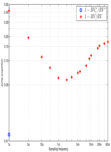
Financial modeling benefits significantly from a nuanced understanding of price fluctuations, moving beyond simple variation measures to incorporate stochastic volatility and asymmetry. Recent research, utilizing five-minute data, reveals a critical refinement in estimating the impact of ‘jumps’ – sudden, large price changes. This analysis demonstrates that the contribution of jumps to overall price variability is substantially lower than previously thought, averaging around 1% compared to the 7-11% suggested by studies relying on lower-frequency data. This more precise jump estimation, combined with models acknowledging fluctuating volatility and the disproportionate impact of negative price shocks, results in more realistic and robust financial models capable of more accurately reflecting market behavior and improving risk assessment.
The pursuit of accurate modeling necessitates a rigorous examination of underlying data structures. This study, revealing a diminished jump component in high-frequency financial data, exemplifies this principle. It demonstrates how prior estimations, based on lower frequencies, obscured the true nature of price movements. As Isaac Newton observed, “If I have seen further it is by standing on the shoulders of giants.” This research builds upon existing knowledge, refining our understanding of market microstructure by utilizing the highest resolution tick data. The apparent jumps previously identified are, in fact, bursts of volatility-a critical distinction achieved through detailed analysis and a commitment to uncovering structural dependencies hidden within the data.
Beyond the Jump
The apparent shrinkage of the jump component as data resolution increases presents a curious challenge. It suggests that much of what has been historically interpreted as discrete price jumps may, in fact, be the high-frequency manifestation of continuous volatility processes. This is not necessarily a refutation of jump-diffusion models, but rather a call for careful consideration of the data’s intrinsic limitations. The field must now grapple with distinguishing between true jumps – those driven by fundamental information – and the illusion of jumps created by the granular nature of market activity.
A crucial next step involves exploring the relationship between pre-averaging intervals and the observed jump size. While higher frequency data reveals a smoother price path, it also increases computational burden. Finding the optimal balance – the point at which statistical power isn’t sacrificed for computational efficiency – remains a significant hurdle. Furthermore, a deeper understanding of the microstructure noise inherent in tick data is paramount. The line between signal and noise is often blurred, and rigorous filtering techniques are needed to avoid masking genuine price discontinuities.
It is worth remembering that visual interpretation requires patience: quick conclusions can mask structural errors. The pursuit of ‘true’ jumps may ultimately be less fruitful than a nuanced understanding of the continuous processes that underpin market dynamics. Perhaps the question isn’t whether jumps exist, but rather how we define – and detect – them in a world of ever-increasing data resolution.
Original article: https://arxiv.org/pdf/2602.10925.pdf
Contact the author: https://www.linkedin.com/in/avetisyan/
See also:
- Top 20 Dinosaur Movies, Ranked
- 20 Movies Where the Black Villain Was Secretly the Most Popular Character
- 25 “Woke” Films That Used Black Trauma to Humanize White Leads
- Celebs Who Narrowly Escaped The 9/11 Attacks
- Silver Rate Forecast
- Spotting the Loops in Autonomous Systems
- Gold Rate Forecast
- 22 Films Where the White Protagonist Is Canonically the Sidekick to a Black Lead
- From Bids to Best Policies: Smarter Auto-Bidding with Generative AI
- Can AI Lie with a Picture? Detecting Deception in Multimodal Models
2026-02-13 01:21